

Create a Pivot Table in Google Sheet
A pivot table is a table summarizing the data or information from other source tables without changing the data in the source table. Normally people are used to creating the pivot table in excel.
But Google sheet also support the formulation and use of pivot table with the amazing user experience.
Google recently introduced “Explore” on google sheet by using machine intelligence. This feature helps the users to ask questions in natural languages relating to our data in the google sheet. When we arrange data in google sheet, the sheet itself suggesting many data analysis resources instantly without doing anything manually in the sheet.
First, we need to create a data table or import a data table in the Google Sheet.

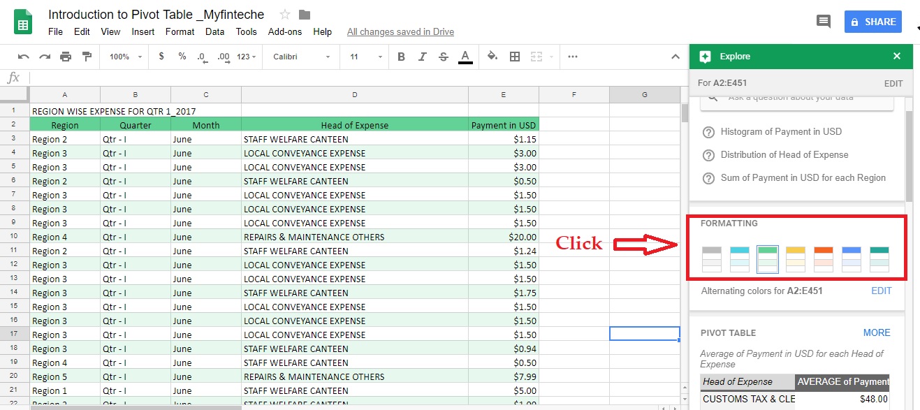
Then we need to just format the table. At the Right bottom, we can see Explore” button along with a star in a green cloured form. Just click on the “Explore”.

Then a rectangular pop up will be shown. There we can find a lot of resources to help the users with regards to the data in Google sheet.
Example: Question bar to ask questions about the data in our natural language, some toilor maid question, formatting area, Pivot table its analysis etc.

Then click the “Formatting” option for a required format of the table.
To create a custom Pivot Table, select the entire table including the heading. Click anywhere in the table, then go to “Data”>”Pivot Table “. This step will create a pivot table in a new sheet.

In the new sheet, we can see the items mentioned below
- Pivot table area
- Auto-suggested pivot table or recommendation from Google sheet
- Area for creating a new pivot table

Once we click the “Rows”, it will display all the row heads, then we need to check the row head we needed

As we needed the pivot table for month wise expense heads, we selected the “Head of Expense” as a row. So just click “ADD” button corresponding to the head

Then we have to create Colum. Click the column button, then click ‘month” then the columns created with the grand total column.

Next, we have to create the value section. Go to “Values”. there we can see an additional option to create a “Calculated Value ” also.

After adding the “Value”, if we wish to add any filter to the table, we add it by clicking the “Filter” button from the bottom, Then the pivot table will form as showing below.

Now we just format the table by adjusting the height or width etc, Our pivot table is ready
Sharing of Pivot Table created in Google sheet
After creating the pivot table, we can share it with others by defining the criteria. Based on the criteria, the person to whom the pivot table shared can view, edit or can comment.
To do that click on the blue “SHARE” button from the top of-of the right side . A pop up will display. Click the “Advanced” button

Then in the new window, select “Can view”, “Can comment” or “Can view” option and enter the email id of the person to whom the link has to be shared. Click “Send” to share.

This is a very basic article regarding the creation of the pivot table in Google sheet. Hope this helps you, people, to understand the concept. If you feel this topic is useful, please do not hesitate to share with your friends also.
You can watch the below video for a better understanding.